Figure 1
Thursday and Friday were both -1.2 foot tides. Our team met on Wednesday night. Thursday was spent rebuilting the cart, dubbed "Beach Comber I", and mounting the GPS antenna. While Bradley worked on the hardware and software to make the Old Laptop Linux Data logger , Jerry worked on the fluxgate magnetometers, and Jon watched the tides so as to make predictions of when and where to go out on the next low tide. One thing we realised is that we could log data from all magnetometers; we implemented these changes. On Friday morning's low tide, we went out to collect data.
Beachcomber I was equipped with 1 Cs magnetometer and three fluxgate magnetometers. These were polled by the data logger at regular intervals. To determine the location of each bit of polled magnetometer data, a differential GPS unit was mounted atop Beachcomber I. For each reading of one of the magnetometers, a position measurement was read from the GPS unit. Data was collected at approximately 1 second intervals (see below for details).
With this set up, we were able to move Beachcomber I in an approximate grid patter, not being too concerned about floolowing an exact grid or maintaining constant speeds.
For coorelation purposes, we took data in lines along the line of sight of the historic photograph and in lines perpendicular to the line of site. (After completing that pattern, we had some time before high tide and sufficient battery power to wonder around a bit for good measure. Hence, the odd 'finger' in the survey pattern.)
Once the data was collected, I used the technique of Radial Basis Functions to take all the magnetometer data taken at random positions on the survey and interpolate them onto a square grid for plotting and further analysis. However, there was concern about gaps in the data when one of another of the instruments wasn't sending data to the data logger.
Below are some plots to help us determine how effective the data collection was. Of course, this doesn't tell us if the data is good, only if there are gaps in the data.
GPS DATA
The GPS didn't record any data for 573 seconds in the middle of the N-S part of the pattern. The cable from the GPS unit to the data logger came loose. This was the only period it failed to send data. That is about 4 transects.
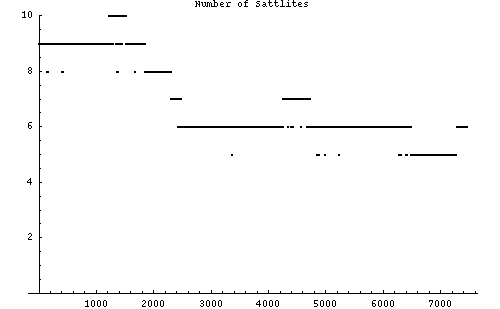
In another place going E-W a lot of GPS data dropped out. Data was coming in intermitantly as if there were fewer satellites or one of our heads was blocking the antenna. The number of satellites is shown in Figure 1 versus the time the GPS data was logged. In all plot versus time, the units are seconds.
Figure 1
The quality of the GPS data generally wasn't very good in that it was only briefly running in differential mode, much of the time it was trying to get a fix as we were trundling along. Figure 2 shows the quality of the data versus the logged time. A value of 4 indicates the GPS was running in differential mode.
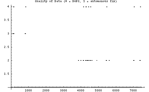
Figure 2
Figure 3
Figure 4
Finally, the position on the survey grid can be computed and plotted for each GPS data location logged. This is seen in Figure 5. In Figure 6, the points are connected, giving a sense of the path taken. The units on the axes are meters.
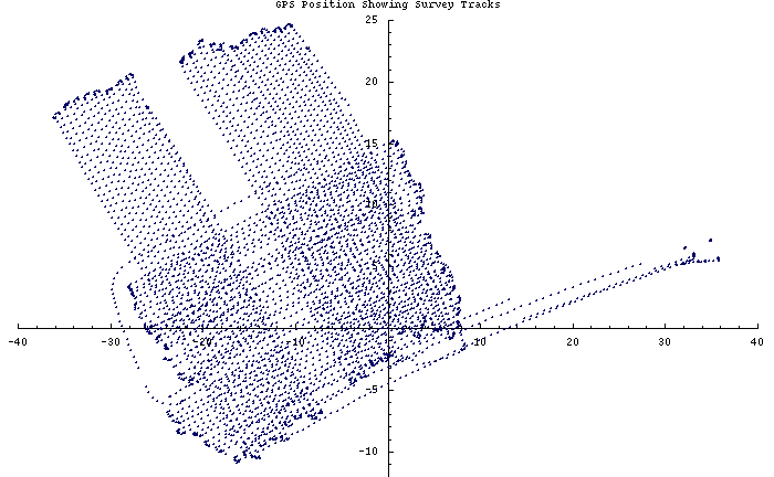
Figure 5
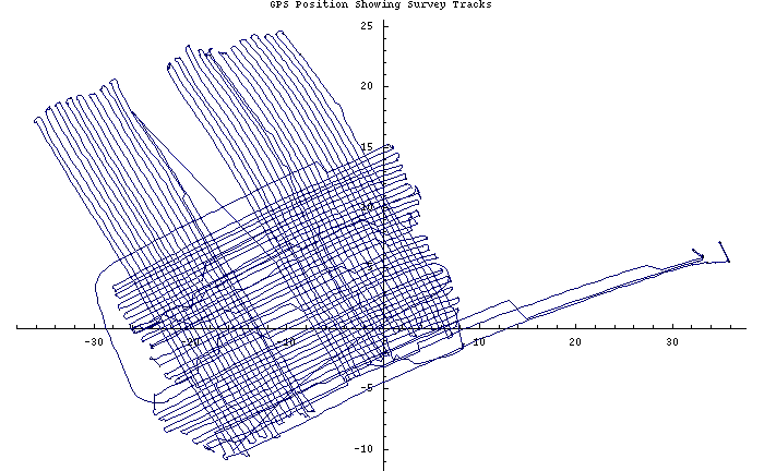
Figure 6
Caesium Magnetometer DATA
We lost about 1500 points of Cs magnetometer data (whilst another cable came unplugged from the data logger). At a data rate of 0.1 Hz, that's 2.5 minutes of data, or about one transect.
The lost data can be seen in a plot of the time tags versus datum number; this is shown in Figure 7. Also, the gap in data is apparent in the plot of the magnetometer data value versus time as seen in Figure 8; also apparent is the change in direction -- N-S tracks versus E-W tracks.
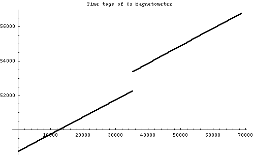
Figure 7
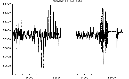
Figure 8
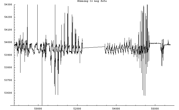
Figure 9
Interpolation was done on the GPS data's time tags and the time tags provided for each magnetometer datum to arrive at a positon on the survey grid. In addition, as this magnetometer was mounted on the front of the cart, a correction was made in the position to reflect the position not of the GPS unit, rather the magnetometer itself. Furthermore, when the data from the GPS was missing, the position of the magetometer is uncertain; such data was removed.
Figure 10 shows the discrete points where a magnetometer datum was taken on the survery grid. Figure 11 shows the path the cart took by connecting these points. Notice the circles at the ends of each track are the result of turning the cart about. Units on the axes are meters.
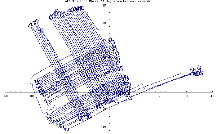
Figure 10
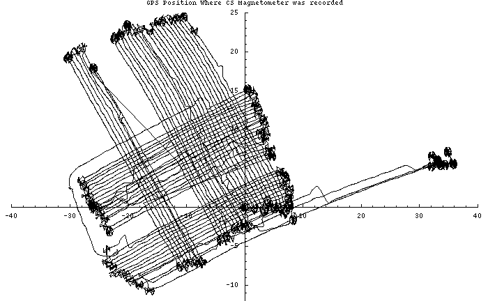
Figure 11
Flux Gate Magnetometer DATA
I don't understand why, but the fluxgate magnetometer data also occationally was missing. It wasn't completely random, there were times when all the data was polled and came in at 0.1 Hz, but sometimes the logger would either suspend polling, or would poll and get no response (in which case it would wait for 100 mS before trying again). In any event, there are times in the survey when lots of data went missing as the effective polling rate when way down. The longest wait was 7 seconds. A scatter plot of the time vs the derivative of the time shows this well, see Figure
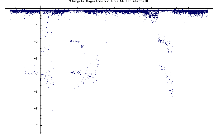
Figure 12
Just for kicks, I plotted each fluxgate magnetometer versus time. Figure 13, 14, and 15 show these plots for magentometer 0, 1, and 2 respectively. (Please ignore the title on the plot, they are incorrect.) The range is 8 bits, so we were not taking advantage of much of the dynamic range available.
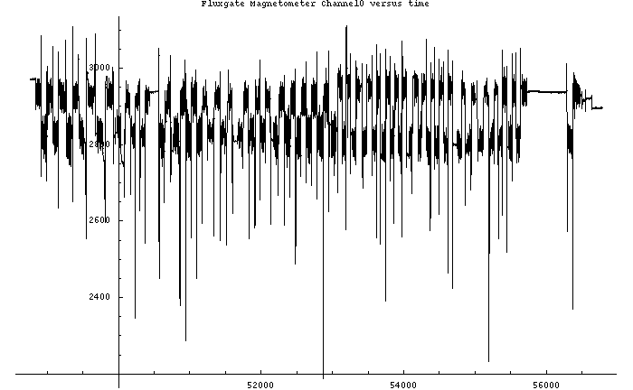
Figure 13: Channel 0

Figure 14: Channel 1

Figure 15: Channel 2
As with the Cs magnetometer, interpolation was done on the GPS data to arrive at a positon on the survey grid for each fluxgate magnetometer's data. Since magnetometer 0 was mounted on the port side front of the cart, magnetmeter 1 and the centre front (just behind the Cs magnetomoeter) and magnetometer 2 on the starboard front, a correction was made in each position to reflect the actual position. Whenever the data from the GPS was missing, the associated magetometer data was removed.
Figures 16, 17, and 18 show the discrete points where a magnetometer datum was taken on the survery grid. Note the gaps in the data.
Figures 19, 20, and 21 show the path the cart took by connecting these points. Notice the circles at the ends of each track are the result of turning the cart about. Units on the axes are meters.
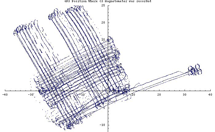
Figure 16: channel -

Figure 17:channel 1
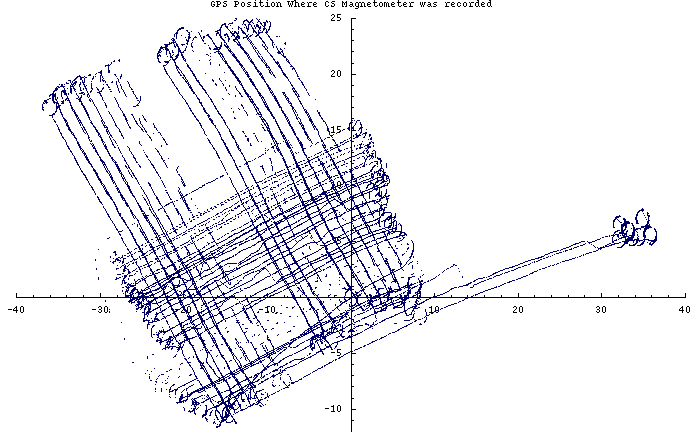
Figure 18:channel 2
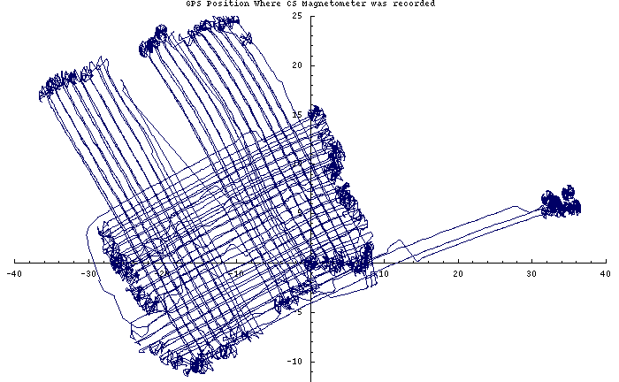
Figure 19:channel 0
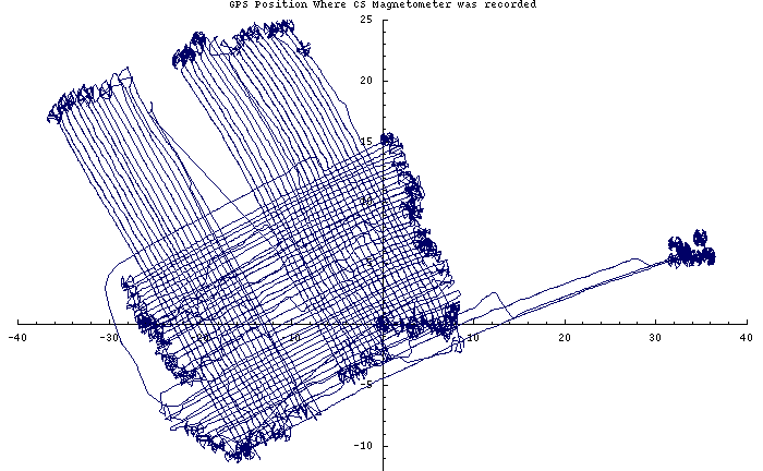
Figure 20:channel 1
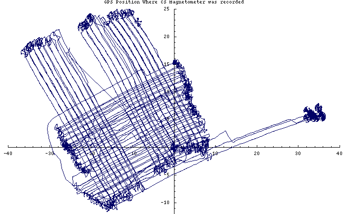
Figure 21:channel 2
Although its completely useless, a 3-D plot of the x-y position on the survery grid versus fluxgate channel 0 is seen in Figure 22.
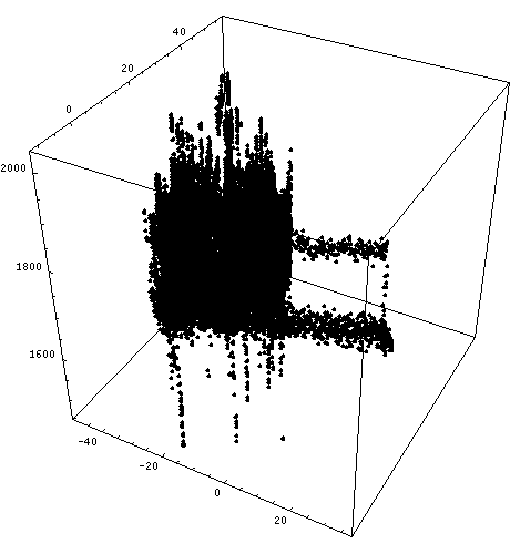
Figure 22